multilayer_witness_fit

esis.flights.f1.optics.gratings.materials.multilayer_witness_fit()

A multilayer stack fitted to the witness sample measurements given by multilayer_witness_measured().

This fit has five free parameters: the ratio of the thicknesses of \(\text{Mg}\), \(\text{Al}\), and the \(\text{SiC}\) to their as-designed thickness, the roughness of the substrate, and a single roughness parameter for all the layers in the multilayer stack.

Examples

Plot the fitted vs. measured reflectivity of the grating witness samples.

import numpy as np
import matplotlib.pyplot as plt
import astropy.units as u
import astropy.visualization
import named_arrays as na
import optika
from esis.flights.f1.optics import gratings

# Load the measured reflectivity of the witness samples
multilayer_measured = gratings.materials.multilayer_witness_measured()
measurement = multilayer_measured.efficiency_measured

# Isolate the angle of incidence of the measurement
angle_incidence = measurement.inputs.direction

# Fit a multilayer stack to the measured reflectivity
multilayer = gratings.materials.multilayer_witness_fit()

# Define the rays incident on the multilayer stack that will be used to
# compute the reflectivity
rays = optika.rays.RayVectorArray(
    wavelength=na.geomspace(250, 950, axis="wavelength", num=1001) * u.AA,
    direction=na.Cartesian3dVectorArray(
        x=np.sin(angle_incidence),
        y=0,
        z=np.cos(angle_incidence),
    ),
)

# Compute the reflectivity of the fitted multilayer stack
reflectivity_fit = multilayer.efficiency(
    rays=rays,
    normal=na.Cartesian3dVectorArray(0, 0, -1),
)

# Plot the fitted vs. measured reflectivity
fig, ax = plt.subplots(constrained_layout=True)
na.plt.scatter(
    measurement.inputs.wavelength,
    measurement.outputs,
    ax=ax,
    label="measurement"
);
na.plt.plot(
    rays.wavelength,
    reflectivity_fit,
    ax=ax,
    axis="wavelength",
    label="fit",
    color="tab:orange",
);
ax.set_xlabel(f"wavelength ({rays.wavelength.unit:latex_inline})")
ax.set_ylabel("reflectivity")
ax.legend();

# Print the fitted multilayer stack
multilayer

MultilayerMirror(
    layers=[
        Layer(
            chemical=Chemical(
                formula='SiC',
                is_amorphous=True,
                table='kortright',
            ),
            thickness=9.60594508 nm,
            interface=ErfInterfaceProfile(
                width=1.90483881 nm,
            ),
            kwargs_plot={'color': 'lightgray'},
            x_label=None,
        ),
        Layer(
            chemical='Al',
            thickness=4.80725357 nm,
            interface=ErfInterfaceProfile(
                width=1.90483881 nm,
            ),
            kwargs_plot={'color': 'lightblue'},
            x_label=1.1,
        ),
        Layer(
            chemical=Chemical(
                formula='Mg',
                is_amorphous=False,
                table='fernandez_perea',
            ),
            thickness=26.62708342 nm,
            interface=ErfInterfaceProfile(
                width=1.90483881 nm,
            ),
            kwargs_plot={'color': 'pink'},
            x_label=None,
        ),
        PeriodicLayerSequence(
            layers=[
                Layer(
                    chemical='Al',
                    thickness=1.20181339 nm,
                    interface=ErfInterfaceProfile(
                        width=1.90483881 nm,
                    ),
                    kwargs_plot={'color': 'lightblue'},
                    x_label=1.1,
                ),
                Layer(
                    chemical=Chemical(
                        formula='SiC',
                        is_amorphous=True,
                        table='kortright',
                    ),
                    thickness=9.60594508 nm,
                    interface=ErfInterfaceProfile(
                        width=1.90483881 nm,
                    ),
                    kwargs_plot={'color': 'lightgray'},
                    x_label=None,
                ),
                Layer(
                    chemical=Chemical(
                        formula='Mg',
                        is_amorphous=False,
                        table='fernandez_perea',
                    ),
                    thickness=26.62708342 nm,
                    interface=ErfInterfaceProfile(
                        width=1.90483881 nm,
                    ),
                    kwargs_plot={'color': 'pink'},
                    x_label=None,
                ),
            ],
            num_periods=3,
        ),
        Layer(
            chemical='Al',
            thickness=12.01813392 nm,
            interface=ErfInterfaceProfile(
                width=1.90483881 nm,
            ),
            kwargs_plot={'color': 'lightblue'},
            x_label=1.1,
        ),
    ],
    substrate=Layer(
        chemical='Si',
        thickness=10. mm,
        interface=ErfInterfaceProfile(
            width=1.00211621 nm,
        ),
        kwargs_plot={'color': 'gray'},
        x_label=None,
    ),
)

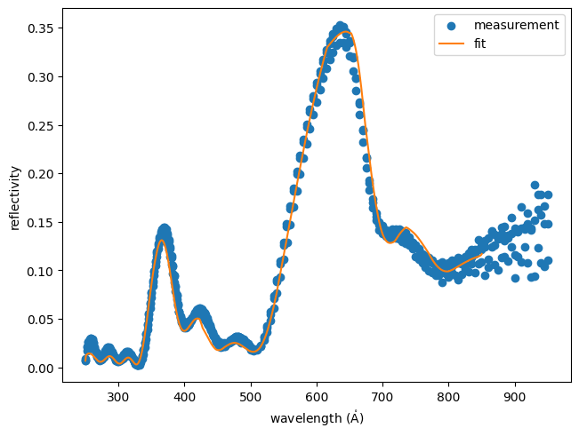
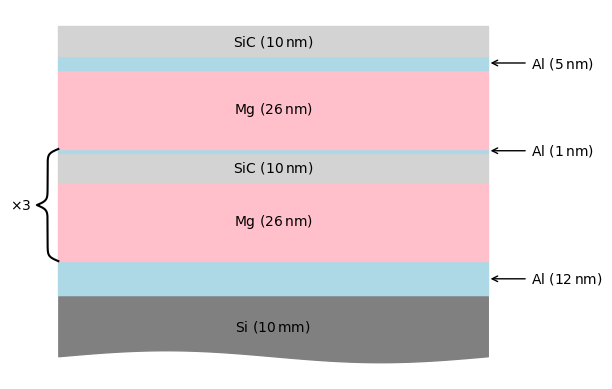
Plot a diagram of the fitted multilayer stack

with astropy.visualization.quantity_support():
    fig, ax = plt.subplots()
    multilayer.plot_layers(
        ax=ax,
        thickness_substrate=20 * u.nm,
    )
    ax.set_axis_off()

Return type:

MultilayerMirror